Article 7: Visualizing with maps
2022-06-09
Source:vignettes/a07_visual_maps.Rmd
a07_visual_maps.RmdWhile ALUES can generate tables for suitability scores and classes, it can also take advantage of the rich mapping library of R. The main requirement of course is the availability of the longitude and latitude for each of the land units. This is possible for Marinduque as it has spatial variables.
Suitability scores and classes
Suppose we want to evaluate the land units for banana, then:
## Loading required package: Rcpp
y <- MarinduqueLT
banana_suit <- suit("banana", terrain=y)
## Warning in suitability(terrain, crop_soil, mf = mf, sow_month = NULL, minimum
## = minimum, : maximum is set to 16 for factor CECc since all parameter intervals
## are equal.
banana_ovsuit <- overall_suit(banana_suit[["soil"]], method="average")Generate maps
There are several ways to generate maps in R, but the following uses ggmap library:
library(ggmap)
library(raster)
library(reshape2)
map_lvl0 <- getData("GADM", country = "PHL", level = 0)
map_lvl2 <- getData("GADM", country = "PHL", level = 2)
prov <- map_lvl2[map_lvl2$NAME_1 == as.character("Marinduque"),]
munic_coord <- coordinates(prov)
munic_coord <- data.frame(munic_coord)
munic_coord$label <- prov@data$NAME_2
val <- banana_suit[["soil"]][[2]]
val["Overall Suitability"] <- banana_ovsuit[,1]
d_map <- melt(as.matrix(val))
d_map$Lon <- rep(y$Lon, ncol(val)); d_map$Lat <- rep(y$Lat, ncol(val))
fill <- "#FFF7BC"; shadow <- "#9ECAE1"; ncol <- 3; size <- 3; alpha <- 1
text_opts <- list(alpha = 1, angle = 0, colour = "black", family = "sans", fontface = 1, lineheight = 1, size = 3)
labels <- list(title = "", xlab = "", ylab = "")
p1 <- ggplot() + geom_polygon(data = prov, aes(long + 0.008, lat - 0.005, group = group), fill = shadow) +
geom_polygon(data = prov, aes(long, lat, group = group), colour = "grey50", fill = fill) +
geom_tile(aes(x = Lat, y = Lon, fill = value), data = d_map, size = size, alpha = alpha) +
facet_wrap(~ Var2, ncol = ncol) +
geom_polygon(data = prov, aes(long, lat, group = group), colour = "#4E4E4C", alpha = 0) +
geom_label(data = munic_coord, aes(x = X1, y = X2, label = label), alpha = 0.5,
angle = text_opts$angle, colour = "white", fill = "black", family = text_opts$family,
fontface = text_opts$fontface,
lineheight = text_opts$lineheight, size = text_opts$size) +
coord_equal() + ggtitle(as.character(labels$title)) + xlab(as.character(labels$xlab)) + ylab(as.character(labels$ylab)) +
scale_fill_gradientn(name = "Score\n", colors = c("red", "#FFDF00")) +
scale_x_continuous(breaks = round(seq(min(d_map$Lat) + 0.05, max(d_map$Lat), len = 3), 2)) +
theme(panel.background = element_rect(fill = '#F7E7CE'),
strip.background = element_rect(fill = "#D4BF96"),
strip.text.x = element_text(size = 12),
axis.text.x = element_text(size=12),
legend.text=element_text(size=12),
legend.title=element_text(size=12),
axis.text.y = element_text(size=12), legend.position = c(0.85, 0.25))
p1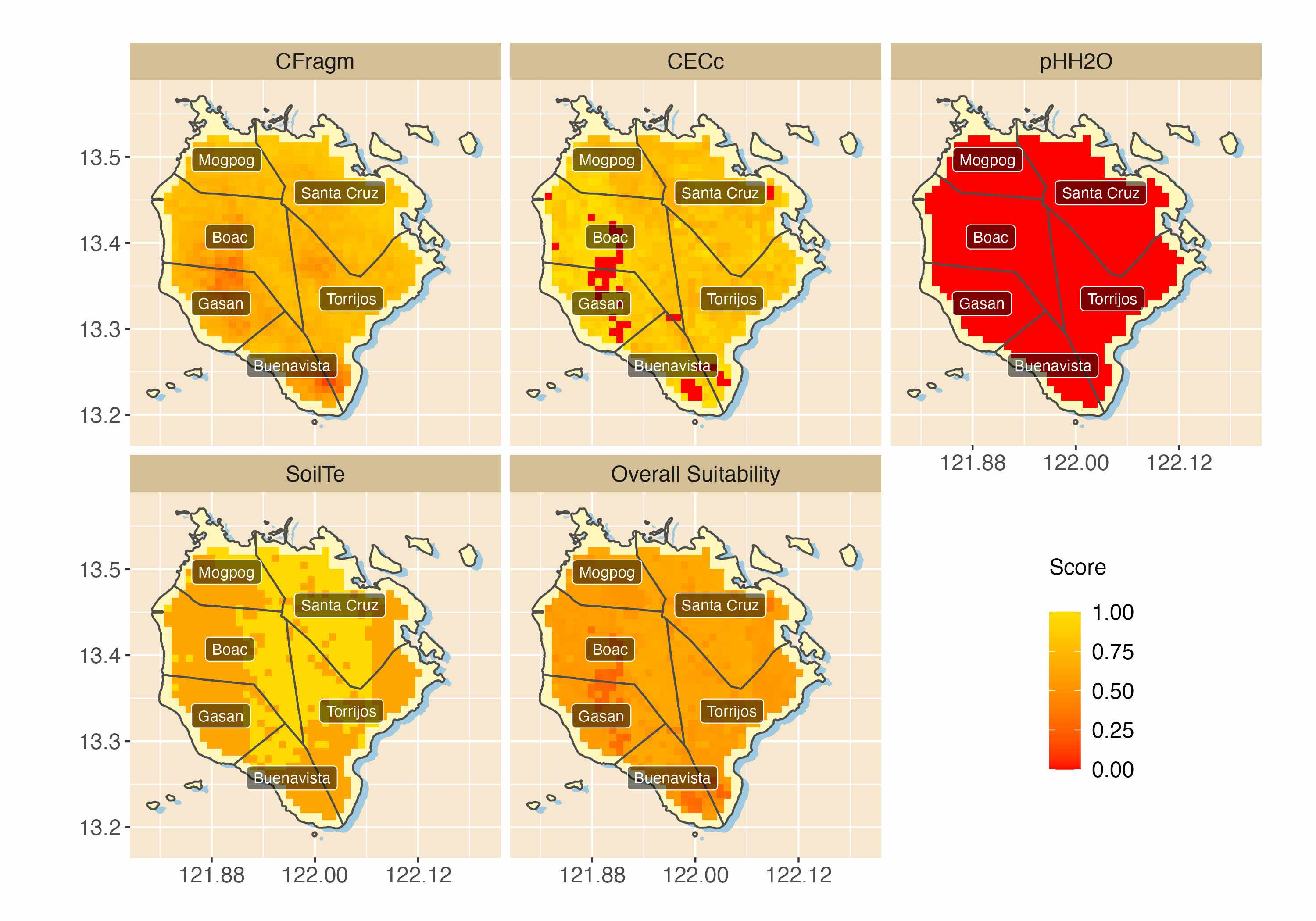 And for
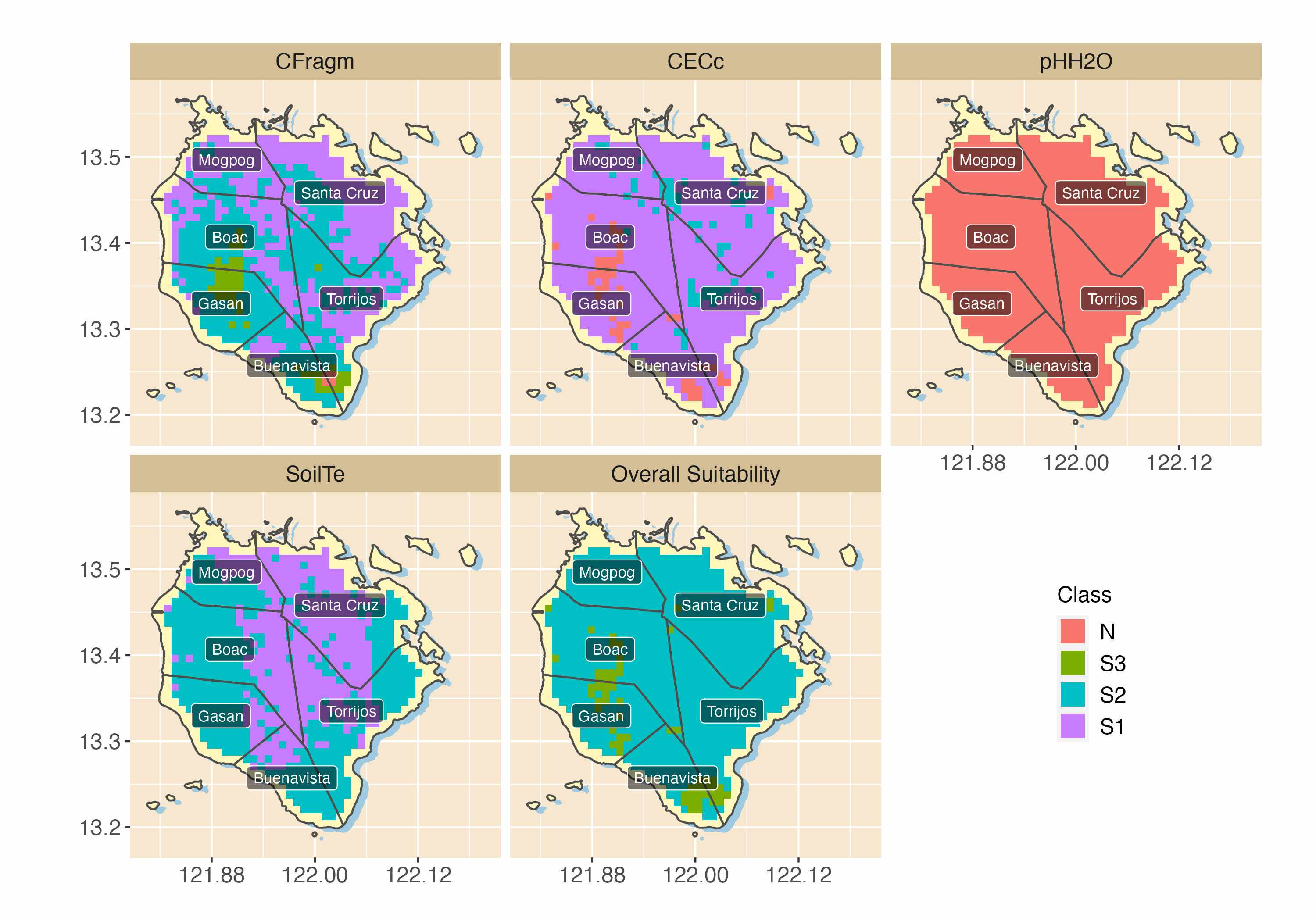
suitability classes:
And for
suitability classes:
val <- banana_suit[["soil"]][[3]]
val["Overall Suitability"] <- banana_ovsuit[,2]
d_map <- melt(as.matrix(val))
d_map$Lon <- rep(y$Lon, ncol(val)); d_map$Lat <- rep(y$Lat, ncol(val))

d_map$Class <- factor(d_map$value, levels=c("N", "S3", "S2", "S1"))

p1 <- ggplot() + geom_polygon(data = prov, aes(long + 0.008, lat - 0.005, group = group), fill = shadow) +
  geom_polygon(data = prov, aes(long, lat, group = group), colour = "grey50", fill = fill) +
  geom_tile(aes(x = Lat, y = Lon, fill = Class), data = d_map, size = size, alpha = alpha) +
  facet_wrap(~ Var2, ncol = ncol) +
  geom_polygon(data = prov, aes(long, lat, group = group), colour = "#4E4E4C", alpha = 0) +
  geom_label(data = munic_coord, aes(x = X1, y = X2, label = label), alpha = 0.5,
             angle = text_opts$angle, colour = "white", fill = "black", family = text_opts$family,
             fontface = text_opts$fontface,
             lineheight = text_opts$lineheight, size = text_opts$size) +
  coord_equal() + ggtitle(as.character(labels$title)) + xlab(as.character(labels$xlab)) + ylab(as.character(labels$ylab)) +
  scale_colour_discrete(name = "Class\n", breaks=c("N", "S3", "S2", "S1"), labels=c("N", "S3", "S2", "S1")) +
  scale_x_continuous(breaks = round(seq(min(d_map$Lat) + 0.05, max(d_map$Lat), len = 3), 2)) +
  theme(panel.background = element_rect(fill = '#F7E7CE'),
        strip.background = element_rect(fill = "#D4BF96"),
        strip.text.x = element_text(size = 12),
        axis.text.x = element_text(size=12),
        legend.text=element_text(size=12),
        legend.title=element_text(size=12),
        axis.text.y = element_text(size=12), legend.position = c(0.85, 0.25))
p1